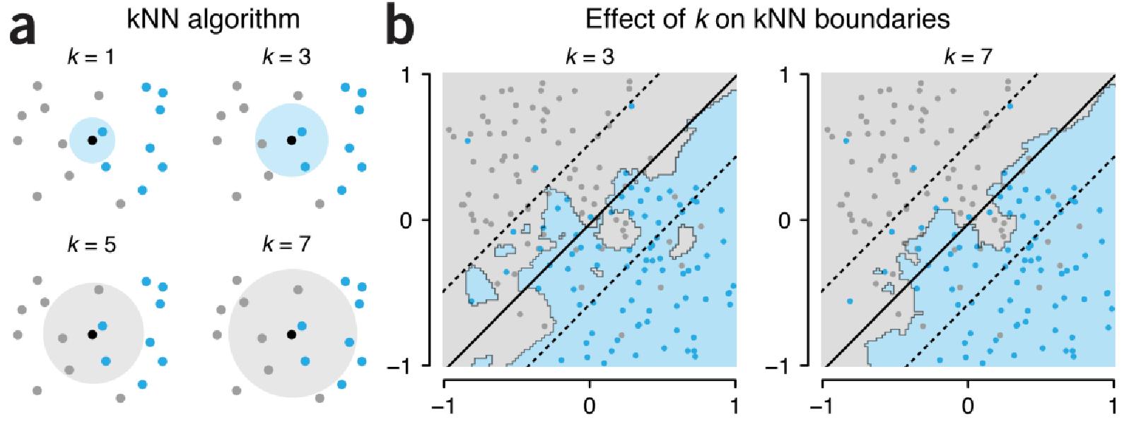
The \(k\)-nearest neighbors algorithm predicts the label of an instance (in machine learning, an instance is a data unit/a sample) by searching, among the training data units (for which the labels are known), the \(k\) instances that are closest to the instance to classify (its nearest neighbors). The algorithm specification is as follows.
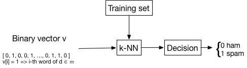
Given a test mail \(m\), normalized and vectorized as described in this page, the spam detector searches the \(k\) nearest neighbors of \(m\) within the set of training instances, all of them with a label (ham or spam), and assigns to \(m\) the majority label among the \(k\) nearest neighbors.
This is the classical \(k\)-nearest neighbors, where the prediction is the most frequent label among these \(k\) nearest neighbors.
More generally, once the \(k\) nearest neighbors of \(v\) are determined, \(\{nn_1, nn_2, ..., nn_k\}\), the label \(y\) for this sample \(v\) is set to 1 if the probability of \(y\) being 1 is over some threshold. Formally, \(k\)-nearest neighbors in binary classification estimates the probability of a class by the following formula: \(\hat{p}(y=1 \mid x) = \frac{1}{k} \sum_{i=1}^{k} y_{nn_i}\). Then, the label \(y\) is given by \(\hat{y} = \begin{cases} 1 \text{ if } \hat{p}(y=1 \mid x) > \text{threshold,} \\ 0 \text{ otherwise.} \end{cases}\)
The majority vote is the special case where threshold \(=0.5\).
You are going to fully implement a \(k\)-NN classifier.
Once the spam detector is implemented, we aim to evaluate its performance. The simplest evaluation method is to compute the error rate, that is, the number of wrongly classified mails over the total number of mails. However, if the dataset contains 95 % of ham mails and only 5 % of spam mails, even if the classifier predicts deterministically ham (non-spam), the error rate will be only 5 %, although this is clearly not a good classifier.
In order to obtain a better evaluation for the spam detector, the confusion matrix is introduced. This matrix considers successes and failures for each label (ham or spam) separately. The confusion matrix that we consider in this TD is defined as follows:
| Predicted label | Spam | Ham | |
|---|---|---|---|
| True label | Spam | true positive (TP) | false negative (FN) |
| Ham | false positive (FP) | true negative (TN) |
The confusion matrix allows to define new estimators: detection rate (also known as recall), error rate, false-alarm rate, precision, and F-score.
\[\begin{equation} \mbox{Detection rate} = \mbox{Recall} = \frac{\textrm{TP}}{\textrm{TP} + \textrm{FN}} \end{equation}\]
\[\begin{equation} \mbox{Error rate} = \frac{\textrm{FP} + \textrm{FN}}{\textrm{FP} + \textrm{FN} + \textrm{TP} + \textrm{TN}} \end{equation}\]
\[\begin{equation} \mbox{False-alarm rate} = \frac{\textrm{FP}}{\textrm{FP} + \textrm{TN}} \end{equation}\]
\[\begin{equation} \mbox{Precision} = \frac{\textrm{TP}}{\textrm{TP} + \textrm{FP}} \end{equation}\]
\[\begin{equation} \mbox{F-score} = \frac{2 \cdot \mbox{Precision} \cdot \mbox{Recall}}{\mbox{Precision} + \mbox{Recall}} \end{equation}\]
In this example, the false-alarm rate is 0 and the precision is 100 %, however, the detection rate (or recall) is 0. Also, the F-score is 0. By way of the harmonic mean, the F-score weights both the false negatives and the false positives.
Statistics relies on the fact that in order to infer a real value (regression) or a label (classification) \(y\) for a new point \(x\), one has already seen observations that are similar to \(x\), i.e., training data that allowed us to derive some kind of function \(\hat{f}\) that acts as a good mapping from \(x\) to \(y\), i.e., \(\hat{y} = \hat{f}(x) \approx y\). In other words, asymptotic properties of estimators \(\hat{f}\) allow us to have some guarantees that \(\hat{y}\) is close to \(y\). These kinds of guarantees come from the fact that in order to be able to generalize well, we have previously seen enough examples in the training set close to \(x\), i.e., the one for which we’re trying to predict \(y\).
Suppose you can generate data to populate the unit interval (the 1-\(d\) cube) and that you draw 100 evenly spaced sample points. The distance between one point and the next is no more than 0.01, so a method like \(k\)-nearest neighbors makes sense: the nearest neighbors are always close to any new point in \([0,1]\).
Now apply the same reasoning to the 10-\(d\) cube: A lattice that has a spacing of 0.01 between adjacent points would require \(100^{10} = 10^{20}=100 \cdot 10^{9} \cdot 10^{9}\) (one hundred billion billion) sample points. Conversely, if you have few points (w.r.t. \(10^{20}\), which can thus already be quite a lot in absolute terms) in 10-\(d\), then there is a good chance that the nearest neighbors of a new point \(x\) in \([0,1]^{10}\) are relatively far away. Are they then relevant in predicting \(y\)?
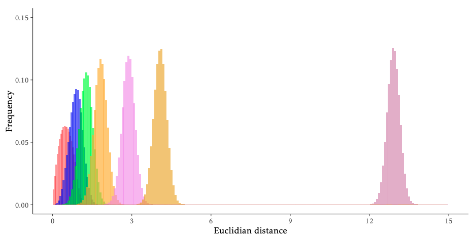
The following figure shows the average Euclidean distance between two random points in the unit cube \([0,1]^d\) for \(d \in \{2, 5, 10, 20, 50, 100, 1000\}\). Remember that our emails live in \(1899-d\).
The relative emptiness of the feature space \(\mathcal{X}\) in high dimensions is not solely a curse. If points are relatively far from each other, there might exist a simple, maybe linear (in \(1899-d\)), decision boundary between spam and ham. In other words, the higher the dimension \(d\), the higher the likelihood of existence of a linear boundary. However, if some feature are just noise w.r.t. the class or contain redundant information, this linear boundary is highly likely to not generalize well, i.e., overfit. To avoid this pitfall but still benefit from the vast amount of available data, a simple solution is to reduce the dimensionality \(d\) of the data to only useful dimensions (in the sense of the predictive task).
It turns out that we can ignore most of the dimensions and your algorithm still (approximately) works!
Say our samples are represented by an \(n \times d\) matrix \(X\). The best setting for the random projection is when \(d\) is greater than \(O(\log(n))\), in particular in the degenerate (for most algorithms, e.g., linear regression) case where \(d > n\). This actually happens in practice: for example, when \(X\) represents several thousands of images, each being a vector in a Euclidean space of size 3 \(\times\) the number of pixels (the 3 comes from the intensities of red, green, and blue (RGB)). A typical setting could be \(n=50{,}000\) images, each having \(d=1920 \cdot 1080 \cdot 3 \approx 6.2 \cdot 10^{6}\) components in \([0,1]\), which would yield a small and fat matrix \(X\).
Given \(\varepsilon \in (0, 1)\), a set \(X\) of \(n\) points in \(\mathbb{R}^{d} = \mathcal{X}\), a number \(\ell> 8 \ln(n)/ \varepsilon^{2}\), and a matrix \(R\) of size \(d \times \ell\), each component of which is sampled from a Gaussian distribution with mean \(0\) and variance \(1 / \ell\), we have with high probability for all \(x_1, x_2 \in \mathcal{X}\) that
\((1- \varepsilon )\|x_1 - x_2\|^{2} \leq \|x_1 \cdot R- x_2 \cdot R\|^{2} \leq (1+\varepsilon) \|x_1 - x_2\|^{2}\).
In other words, if we lose exponentially many dimensions (in terms of the number \(n\) of data points), we still get approximately the same Euclidean metric on the projection space \(\mathcal{R}\) as we have on \(\mathcal{X}\). If this isn’t magic enough for you, then observe that \(\ell\) is independent of the original number \(d\) of dimensions!
The sketch of the proof is that the random quantity \(\|x_1 \cdot R - x_2 \cdot R \|^2\) has the same mean as \(\|x_1 - x_2 \|^2\) and a certain variance. Because of the Gaussian distribution, this variance decreases exponentially. Hence, it suffices to consider a logarithmic number of dimensions to make sure the variance is small enough, which amounts to achieving a good accuracy. A more formal proof is given in an earlier version of an INF442 TD.
This result can even be improved: The random matrix \(R\) can be sampled from a Rademacher distribution, i.e., \(\begin{cases} - \sqrt{\frac{3}{\ell}} &\text{ with probability } \frac{1}{6}, \\ \sqrt{\frac{3}{\ell}} &\text{ w. p. } \frac{1}{6}, \\ 0 &\text{ w. p. } \frac{2}{3} \end{cases}\), such that the resulting matrix \(R\) is sparse (it has a lot of 0 coefficients, which don’t take space in memory; we only store the non-zero entries).
If you’re interested, you can have a look at scikit-learn’s help page.