This assignment will be closed on May 27, 2026 (23:59:59).

You must be authenticated to submit your files

CSE 102 – Tutorial 11 – Functional programming

Tail recursion and conversion to purely functional code
Programming with binary trees, revisited

Sections tagged with a green marginal line are mandatory.

Sections tagged with an orange marginal line are either more advanced or supplementary, and are therefore considered optional. They will help you deepen your understanding of the material in the course. You may skip these sections on a first pass through the tutorial, and come back to them after finishing the mandatory exercises.

Discussion of the tutorials with friends and classmates is allowed, with acknowledgment, but please read the Moodle page on “Collaboration, plagiarism, and AI”.

We expect you to write your solutions to all of the problems for this tutorial in a file named fun.py and to upload it using the form below. You can resubmit your solution as many times as you like.

Upload form is only available when connected

Tail recursion and conversion to purely functional code

Since Python does not have tail-call optimization, we will need to raise the recursion limit for this section.

import sys
sys.setrecursionlimit(100000)

Recall the example of iterative and recursive versions of Euclid’s algorithm from Lecture 1:

def gcd_it(a,b):
    while b > 0:
        a,b = b,a%b
    return a

def gcd_rec(a,b):
    if b == 0:
        return a
    return gcd_rec(b,a%b)

Up to minor operational details, these two versions of the algorithm have very similar executions. Notice that in the recursive version, the recursive call to gcd_rec(b,a%b) is a tail call, in the sense that the value returned by the recursive call is not modified, and is just passed along as the result of the function.

In contrast, consider the following iterative and recursive versions of the factorial function:

def fact_it(n):
    p = 1
    while n > 0:
        p *= n
        n -= 1
    return p

def fact_rec(n):
    if n == 0:
        return 1
    else:
        return n * fact_rec(n-1)

Although both of these are correct implementations of the factorial function \(n! = n\cdot (n-1)\cdots 1\) and have the same input-output behavior, their flow of execution is different. In fact, they perform the multiplications in opposite orders: the iterative version multiplies from left-to-right (e.g., fact_it computes 4! = 24 by performing the series of multiplications (((1*4)*3)*2)*1), while the recursive version multiplies from right-to-left (e.g., fact_rec computes 4! by performing the series of multiplications 4*(3*(2*(1*1)))). Notice that in the recursive version, the call to fact_rec(n-1) is not a tail call.

Write a tail-recursive version of factorial that mimics the behavior of fact_it by introducing an extra argument p (called an “accumulator”) that represents the running product:
```
def fact_acc(n, p) -> int:
    pass
```
Calling fact_acc(n, 1) should return the same value as fact_it(n), i.e., n!, but the definition of fact_acc should use only tail recursive calls and no iteration.
Can you find a simple formula for the value of fact_acc(n, p) for arbitrary integers p and n >= 0? State your answer as a comment, together with a justification of why the formula is correct.

Recall the n-queens problem as discussed in the lecture on backtracking. The generator function queens(qs, n) below yields all solutions to the n queens problem that extend a partial solution qs represented as a list of integers between 0 and n-1. (This is the same code as seen in class, but with added type annotations for documentation.)

from typing import Iterator

def queens(qs: list[int], n: int) -> Iterator[list[int]]:
    if len(qs) == n:
        yield qs
        return
    for r in range(n):
        # check for row conflict
        if r in qs: continue
        # check for "/" diagonal conflict (same row - column)
        if any(qs[i]-i == r-len(qs) for i in range(len(qs))): continue
        # check for "\" diagonal conflict (same row + column)
        if any(qs[i]+i == r+len(qs) for i in range(len(qs))): continue
        # extend board and recursively generate solutions
        yield from queens(qs + [r], n)

For example, below we use this backtracking solver to extract two solutions to the 8-queens problem:

In [1]: g = queens([], 8)

In [2]: next(g)
Out[2]: [0, 4, 7, 5, 2, 6, 1, 3]

In [3]: next(g)
Out[3]: [0, 5, 7, 2, 6, 3, 1, 4]

The aim of the following optional exercises is to see how generators can be replaced by the use of higher-order functions.

For simplicity, in the first version below we ask you to write a purely functional backtracking solver that looks for a single solution to the n-queens problem, rather than all solutions.

Write a function queens_one(qs, n, ksucc, kfail) of the following type:
```
from typing import Callable

def queens_one[T](qs: list[int], n: int, ksucc: Callable[[list[int]], T], kfail: Callable[[], T]) -> T:
    pass
```
Here the arguments ksucc and kfail are functions called the “success continuation” and “failure continuation”, which the higher-order function queens_one should invoke in the case of success and failure respectively. More precisely, the specification of queens_one is as follows: if there is a solution sol to the n-queens problem extending qs, then it should call and return the value of ksucc(sol); otherwise, it should call and return the value of kfail().

You should write queens_one as a pure recursive function, without using iteration or generators (and certainly without using queens!).

Examples:
```
In [4]: queens_one([], 8, lambda sol : sol, lambda : print('No solution'))
Out[5]: [0, 4, 7, 5, 2, 6, 1, 3]

In [6]: queens_one([], 3, lambda sol : sol, lambda : print('No solution'))
No solution
```
Guidance: you can start by copying the code for the generator function queens, and begin transforming it. The yield operation (yield qs) should be replaced by an appropriate function call (return ksucc(qs)), and you can get rid of the for-loop by an appropriate use of recursion (feel free to introduce any auxiliary functions that you need). Finally, you should think carefully about how to construct the success and failure continuations ksucc and kfail in recursive calls to queens_one (you may want to use lambda syntax).

Now we want to extend the higher-order backtracking solver to generate all solutions. For this it suffices to provide the success continuation an extra argument, which is itself a continuation that can be invoked to retrieve more solutions.

Write a function queens_all(qs, n, ksucc, kfail) of the following type:
```
def queens_all[T](qs: list[int], n: int, ksucc: Callable[[list[int], Callable[[], T]], T], kfail: Callable[[], T]) -> T:
    pass
```
The specification of queens_all is almost the same as for queens_one, but now in the event that there is a solution sol to the n-queens problem extending qs, queens_all(qs, n, ksucc, kfail) should invoke ksucc(sol, krest), where krest is a function (of no arguments) that can be applied krest() to generate all remaining solutions.

As an example, you should be able to generate a list of all solutions to the n-queens problem by calling queens_all with appropriate success and failure continuations, as shown below.
```
In [7]: queens_all([], 4, lambda sol, krest : [sol] + krest(), lambda : [])
Out[7]: [[1, 3, 0, 2], [2, 0, 3, 1]]

In [8]: queens_all([], 6, lambda sol, krest : [sol] + krest(), lambda : [])
Out[8]: [[1, 3, 5, 0, 2, 4], [2, 5, 1, 4, 0, 3], [3, 0, 4, 1, 5, 2], [4, 2, 0, 5, 3, 1]]
```

Programming with binary trees, revisited

Throughout this section we will work with leaf-labelled binary trees, as discussed in class. We recall the encoding below — for simplicity, we assume that all leaves are labelled by integers.

class Leaf:
    def __init__(self, value: int):
        self.value = value
    def __repr__(self):
        return f'Leaf({self.value})'

class Node:
    def __init__(self, left: 'Tree', right: 'Tree'):
        self.left = left
        self.right = right
    def __repr__(self):
        return f'Node({self.left}, {self.right})'

type Tree = Leaf | Node
# (if the above line gives you a syntax error, remove "type" from the previous line, i.e., replace by the following:)
# Tree = Leaf | Node

You should copy these definitions into a file named trees.py. (Or alternatively, download the file here.) Then you should add the line

from trees import Leaf, Node, Tree

to your main source file.

For example, the values

example1 : Tree = Node(Leaf(0), Node(Leaf(1), Leaf(2)))
example2 : Tree = Node(Node(Leaf(0), Leaf(1)), Leaf(2))
example3 : Tree = Node(Node(Node(Leaf(0), Leaf(1)), Leaf(2)), Node(Leaf(3), Leaf(4)))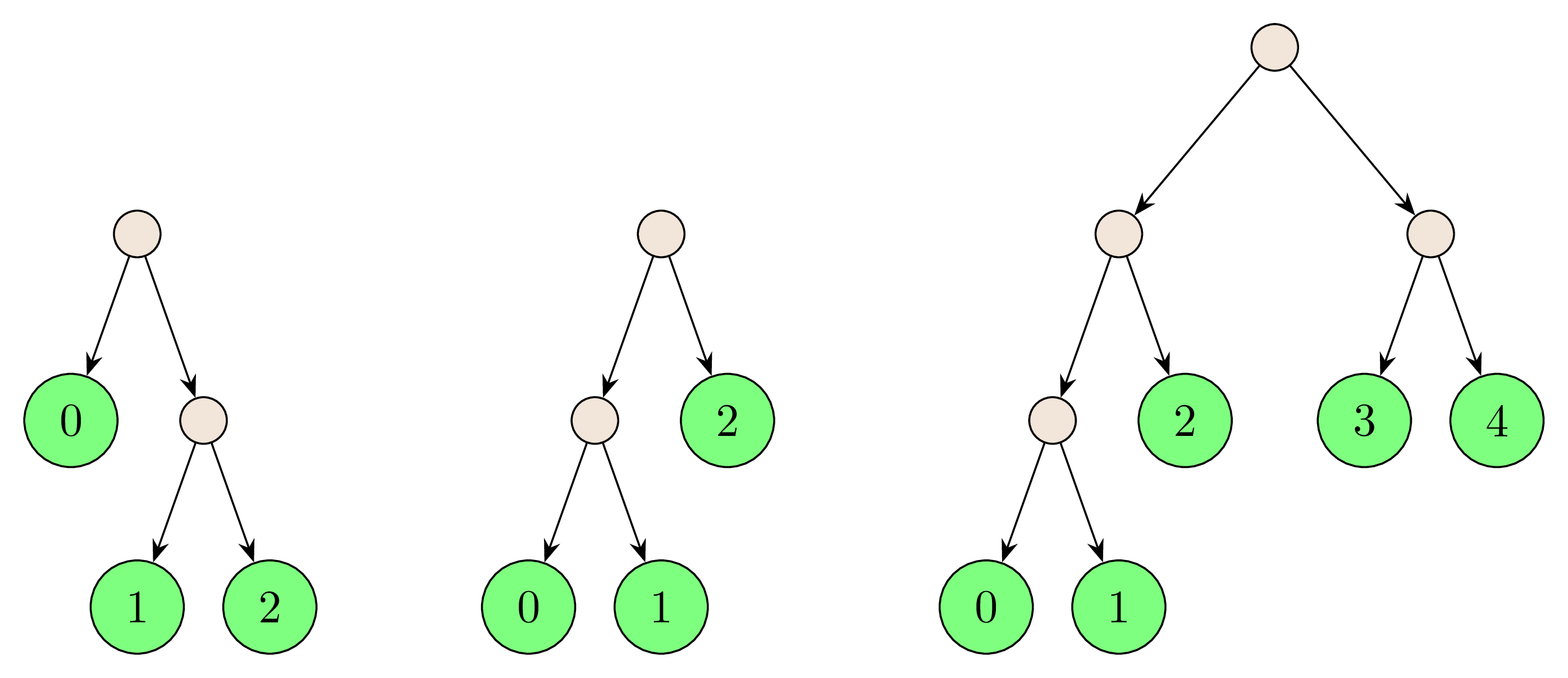

correspond to the three trees below, diagrammatically:

Also useful for testing purposes, the function cbt(n, x=0) defined below constructs a complete binary tree with \(2^n\) leaves labelled from \(x\) to \(x+2^n-1\).

def cbt(n: int, x: int = 0) -> Tree:
    if n == 0: return Leaf(x)
    else:      return Node(cbt(n-1, x), cbt(n-1, x + 2**(n-1)))

Pattern-matching and folds

Making use of recursion and structural pattern-matching (i.e., Python’s match ... case ... syntax), write four functions count_nodes(t), sum_leaves(t), leaves(t), and mirror(t) with the following specifications:
- count_nodes(t: Tree) -> int returns the number of binary nodes in the tree t;
- sum_leaves(t: Tree) -> int returns the sum of the labels of the leaves in the tree t;
- leaves(t: Tree) -> list[int] returns the list of leaf labels in the tree t, listed from left to right;
- mirror(t: Tree) -> Tree returns the mirror image of the tree t.
Examples:
```
In [9]: [(count_nodes(t), sum_leaves(t), leaves(t), mirror(t)) for t in [example1,example2,example3]]
Out[9]: [(2, 3, [0, 1, 2], Node(Node(Leaf(2), Leaf(1)), Leaf(0))),
           (2, 3, [0, 1, 2], Node(Leaf(2), Node(Leaf(1), Leaf(0)))),
           (4,
            10,
            [0, 1, 2, 3, 4],
            Node(Node(Leaf(4), Leaf(3)), Node(Leaf(2), Node(Leaf(1), Leaf(0)))))]

In [10]: [count_nodes(cbt(n)) for n in range(10)]
Out[10]: [0, 1, 3, 7, 15, 31, 63, 127, 255, 511]
```
Warning: Make sure that you have imported the definitions of the tree classes from the trees module as per the above instructions, rather than copying them into your fun.py file. If you do the latter then your code will not pass the testing server!

You probably implemented all four functions from the previous exercise in a very similar way. In fact, they can all be written as folds over a binary tree in the following sense.

Write a higher-order function fold_tree(t, f_leaf, f_node) which takes as input a binary tree t, a unary function f_leaf, and a binary function f_node, and computes a value as follows: the function f_leaf is applied to obtain a value for each leaf label, and these values are combined by using f_node at every binary node. For example, fold_tree(example1, g, h) should evaluate to h(g(0), h(g(1), g(2))) for any functions g and h.

Examples:
```
In [11]: fold_tree(cbt(4), lambda x:x, min)
Out[12]: 0

In [13]: fold_tree(cbt(4), lambda x:x, max)
Out[14]: 15
```

If you have not already done so, add type annotations to your definition of fold_tree, trying to write a type for the function that is as general as possible.

Reimplement the four functions that you defined above, but now just in terms of fold_tree. You should do so by defining the functions f_leaf* and f_node* referenced below or by replacing them with appropriate lambda expressions.

def count_nodes_as_fold(t: Tree) -> int:
    return fold_tree(t, f_leaf1, f_node1)

def sum_leaves_as_fold(t: Tree) -> int:
    return fold_tree(t, f_leaf2, f_node2)

def leaves_as_fold(t: Tree) -> list[int]:
    return fold_tree(t, f_leaf3, f_node3)

def mirror_as_fold(t: Tree) -> Tree:
    return fold_tree(t, f_leaf4, f_node4)

Again just using fold_tree and without making use of any auxiliary recursion, define a function eq_tree(t: Tree, u: Tree) -> bool that determines whether or not two trees t and u are structurally equal.

Examples:
```
In [15]: example1 == Node(Leaf(0), Node(Leaf(1), Leaf(2)))
Out[15]: False

In [16]: eq_tree(example1, Node(Leaf(0), Node(Leaf(1), Leaf(2))))
Out[16]: True

In [17]: eq_tree(example2, Node(Leaf(0), Node(Leaf(1), Leaf(2))))
Out[17]: False
```
Hint: it may help to first define eq_tree using recursion and pattern-matching, before trying to define it as a fold. It is important to keep in mind that fold_tree can compute a value of arbitrary type, in particular it can return a function as its answer.

Rémy’s algorithm

Rémy’s algorithm is a simple and elegant iterative algorithm for generating random binary trees of a fixed size. It is a uniform generator in the sense that every binary tree is generated with equal probability.

At a high level, the algorithm can be described as follows:

Start: a tree with one leaf with label 0.
For i from 1 to n:
1. Choose one existing subtree u at random. (There are 2n+1 subtrees when the tree has n internal nodes.)
2. Toss a coin.
  1. If Heads, make u the left child of a new internal node; attach a new leaf with label i as the right child of the new internal node.
  2. If Tails, do the symmetric thing: u goes on the right and the new leaf with label i goes on the left of a new internal node.

Here is a little animation of Rémy’s algorithm being used to generate a random binary tree with 16 leaves, followed by running the algorithm in reverse to deconstruct the tree:

Observe that as we grow new leaves, we also label them in the order of creation.

Write a function remy(n: int) -> Tree which uses Rémy’s algorithm to generate a uniformly random binary tree with \(n\) binary nodes and \(n+1\) leaves, with the leaves labelled \(0,\dots,n\) in order of creation.

Examples:
```
In [18]: remy(8)
Out[18]: Node(Node(Node(Node(Node(Leaf(7), Node(Leaf(3), Leaf(1))), Node(Leaf(2), Leaf(6))), Leaf(5)), Leaf(8)), Node(Leaf(0), Leaf(4)))

In [19]: remy(8)
Out[19]: Node(Leaf(1), Node(Leaf(2), Node(Node(Leaf(0), Leaf(5)), Node(Node(Leaf(8), Leaf(4)), Node(Leaf(7), Node(Leaf(6), Leaf(3)))))))
```
Hint: to facilitate the step of picking a random subtree u of t and replacing it by a larger tree Node(Leaf(k), u) or Node(u, Leaf(k)), begin by writing a function that enumerates every subtree together with a pointer from its immediate parent. More precisely, write a generator function subtrees(t: Tree, pt: Node, lct: bool) -> Iterator[tuple[Tree, Node, bool]] with the following specification: subtrees(t, pt, lct) generates all triples (u, p, lc) such that u is a subtree of t, p is the immediate parent of u in t, and lc is True just in case u is the left child of p, under the assumption that t = pt.left if lct = True, and t = pt.right if lct = False. Then you can write remy(n) by repeatedly calling subtrees and updating the tree appropriately. To simplify the code, it may help to begin by creating a tree with a dummy binary node at the root and a leaf labelled 0 as (say) its right child.